Debugging Guide

Warning: You should only use these tools actively while debugging and preferably only in simulation, because it slows down the control loop.

When a motion does the wrong thing — or the controller fails to produce a command at all — you need to see what Giskard is computing internally. This guide covers three tools, each answering a different question:

• Debug expressions let you track any symbolic expression (a scalar or a spatial type) that a node computes, so you can watch it change over time.

  • Visualize them live in RViz to answer “where is this point/vector/pose right now, and where does the goal want it?”

  • Plot them to a PDF to answer “how did this value evolve over the whole motion?”

• The QuadraticProgramDebugger answers “why did the QP behave this way?” — it labels the raw solver arrays with constraint and degree-of-freedom names so you can read bounds, weights, and constraint violations by name.

Debug expressions

A DebugExpression (giskardpy.motion_statechart.graph_node.DebugExpression) wraps three things:

• a name, used as the label in every debugging tool,

• an expression — either a Scalar or a spatial type (Point3, Vector3, Quaternion, RotationMatrix, HomogeneousTransformationMatrix, or Pose), and

• a color, used when the expression is rendered.

A node registers a debug expression by appending it to artifacts.debug_expressions inside its build_artifacts() method:

from semantic_digital_twin.world_description.geometry import Color
from giskardpy.motion_statechart.graph_node import DebugExpression

artifacts.debug_expressions.append(
    DebugExpression(
        name=f"{self.name}/current_normal",
        expression=root_V_tip_normal,
        color=Color.from_rgba(red=1, green=0, blue=0, opacity=1),
    )
)

See tasks/align_planes.py for a worked example. For Cartesian tasks there is a convenience helper, CartesianTask.add_goal_and_current_debug_expressions(artifacts, goal, current) (tasks/cartesian_tasks.py), which registers <task name>/goal (green) and <task name>/current (red) so the two can be told apart in RViz.

Every node’s debug expressions are gathered through DebugExpression.collect_from(statechart); the visualizer and plotter below consume that list, so you only have to register the expression once.

Note

Plain Scalar expressions are plotted but not drawn in RViz — only spatial types become markers. Use the plotter to inspect scalars.

Visualizing debug expressions in RViz

The DebugExpressionPublisher (giskardpy.motion_statechart.debug_expression_publisher) turns every spatial-typed debug expression into an RViz marker and republishes it whenever the world state changes.

You do not construct it directly. Instead, add the DebugExpressionPublishing extension to the executor:

from cramph.context import StatechartContext
from cramph.executor import StatechartExecutor
from giskardpy.motion_control import MotionControl
from giskardpy.motion_statechart.debug_expression_publisher import (
    DebugExpressionPublishing,
)
from giskardpy.motion_statechart.ros_context import RosNodeAccess

executor = StatechartExecutor(
    context=StatechartContext(world=world),
    extensions=[RosNodeAccess(node), MotionControl(), DebugExpressionPublishing(node)],
)
executor.compile(motion_statechart)

On compile(), the extension builds the publisher and attaches it to the statechart. Each expression’s name becomes the marker namespace and label, so individual expressions can be toggled on and off in RViz’s display tree. Vector3 expressions are anchored to their visualisation_frame so the arrow is drawn at the right body.

This is the right tool for spatial reasoning: comparing a goal pose against the current pose, checking which way a normal points, or confirming a point is where you expect it in the world.

Each spatial type renders as a different marker, and the <task name>/goal (green) / <task name>/current (red) convention makes the comparison easy to read:

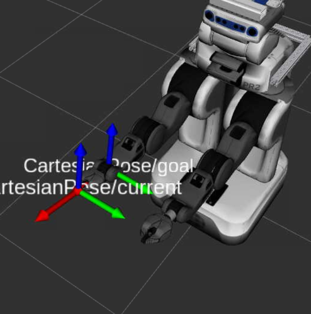
Fig. 1 A Pose is drawn as a coordinate frame. Here CartesianPose/goal and CartesianPose/current show the target and actual end-effector pose side by side.

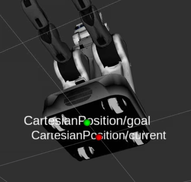
Fig. 2 A Point3 is drawn as a sphere — CartesianPosition/goal (green) and CartesianPosition/current (red).

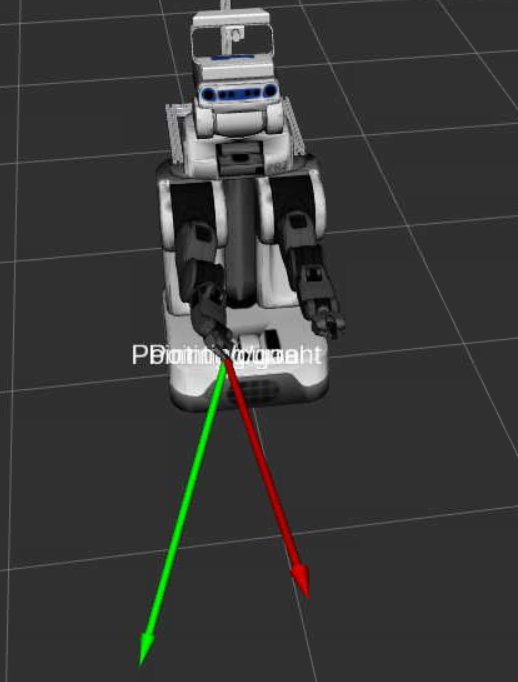
Fig. 3 A Vector3 is drawn as an arrow anchored to its visualisation_frame. Here the green Pointing/goal and red Pointing/current arrows show where the robot should point versus where it currently points.

Plotting debug expressions

To see how debug expressions evolve over an entire motion, add a DebugExpressionRecording (giskardpy.motion_control) to the executor, after MotionControl. It holds a DebugExpressionTrajectoryPlotter (giskardpy.motion_statechart.plotters.debug_expression_trajectory_plotter):

from cramph.context import StatechartContext
from cramph.executor import StatechartExecutor
from giskardpy.motion_control import DebugExpressionRecording, MotionControl

executor = StatechartExecutor(
    context=StatechartContext(world=world),
    extensions=[MotionControl(), DebugExpressionRecording()],
)
executor.compile(motion_statechart)
executor.tick_until_end()
executor.require_extension(DebugExpressionRecording).plotter.plot(
    "./debug_expressions.pdf"
)

The lifecycle is:

• compile() calls the plotter’s reset(...), which builds a fresh trajectory from DebugExpression.collect_from(statechart) and discards any previous recording.

• Every tick() appends the value of each expression after the commands of that tick were applied.

• plotter.plot(file_name) writes the PDF. require_extension raises MissingExecutorExtensionError if the executor has no DebugExpressionRecording.

The plot has one subplot per expression and one line per scalar component, sharing a common time axis — for example a Point3 produces four lines (its homogeneous x, y, z, w components). The plotter exposes a few layout knobs: subplot_height_in_cm, second_width_in_cm, and legend.

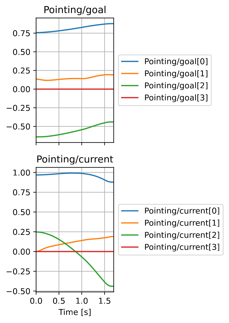
Fig. 4 An example plot for a pointing task: the Pointing/goal and Pointing/current Vector3 expressions, each split into their four homogeneous components, show the goal vector and the current vector converging over the motion.

For a runnable end-to-end example, see test/giskardpy_test/test_motion_statechart/test_debug_expression_trajectory.py.

Inspecting the QP with QuadraticProgramDebugger

When implementing new motion statechart nodes, the controller may produce an unintended command, runs into limits, or the solve fails. To debug this, it may help to look directly into the quadratic program (QP) itself. The QP is just large, anonymous numeric arrays; the QuadraticProgramDebugger (giskardpy.qp.qp_debugger) re-labels those arrays with the corresponding constraint and degree-of-freedom names and exposes them as pandas.DataFrames, so you can read the problem by name.

Every QPController builds one automatically as controller.debugger (with no solution yet). To inspect it:

• you should run the program in debug mode

• place a break point in the last line of QPController.compute_command(...)

• add a watch saying self.debugger.update(solution) (when the solve fails, use update(None))

• look at self.debugger in the debugger

Reading the output

The debugger produces five labeled frames:

• direct_limits — one row per free variable, with its lower/upper box bounds, the solution value, and its quadratic and linear weight. Use it to spot a variable pinned at a bound, a zero or oversized weight, or a solution that landed outside its box. Constraints with a weight of 0 are inactive and will have nan values.

• equality_constraints — columns for the constraint value (matrix × decision variables, excluding slack), the slack (bounds − value, i.e. how much the constraint is violated), and the bounds. A large slack pinpoints the violated equality constraint by name.

• inequality_constraints — same as the previous, but for inequality constraints.

• equality_matrix / inequality_matrix — the labeled constraint matrices (rows are constraint names, columns are degree-of-freedom names). It’s essentially a Jacobian matrix, so look at how degrees of freedom influence your constraints. 0 means no influence, a positive value means increasing the value will also increase constraints’ expression, a negative value means decreasing the value will increase the constraints’ expression.