Graph of Convex Sets

This notebook walks through the way the semantic world navigates spaces that are challenging to navigate. Usually, navigation is done in spaces that are convex, meaning that every point is reachable via a straight line without collision. Unfortunately, the real world is not like this.

The semantic world internally represents the objects in the world using some implementation of a scene description format. These formats include collision information for every object. The collision information is often approximated using a set of boxes.

These collision boxes are converted to their algebraic representation using the random-events package. This allows the free space to be formulated as the complement of the belief state collision boxes. The complement itself is a finite collection of (possible infinitely big) boxes that do not intersect. These boxes, however, have surfaces that are adjacent. Representing this adjacency is done using a Graph of Convex Sets (GCS) where every node is a box, and every edge means that these boxes are adjacent. Navigating the free space is then possible using path finding algorithms on the graph.

You can read more about GCS here.

Let’s get hands on! First, we need to create a world that makes navigation non-trivial.

from semantic_world.world_description.geometry import Box, Scale, Color
from semantic_world.world_description.shape_collection import ShapeCollection, BoundingBoxCollection
from semantic_world.world_description.world_entity import Body
from semantic_world.datastructures.prefixed_name import PrefixedName
from semantic_world.spatial_types import TransformationMatrix
from semantic_world.world import World

box_world = World()

with box_world.modify_world():
    box = Body(name=PrefixedName("box"), collision=ShapeCollection([Box(scale=Scale(0.5, 0.5, 0.5),
                                                        color=Color(1., 1., 1., 1.),
                                                        origin=TransformationMatrix.from_xyz_rpy(0,0,0,0,0,0),)],
                                                        ))
    box_world.add_kinematic_structure_entity(box)
    

Next, we create a connectivity graph of the space so we can solve navigation problems. To visualize the result in a better way, we limit the search space to a finite set around the box. Furthermore, we constraint the robot to be unable to fly by constraining the z-axis. Otherwise, he would get the idea to go over the box, which is not a good idea.

from random_events.interval import SimpleInterval
from semantic_world.world_description.graph_of_convex_sets import GraphOfConvexSets
from semantic_world.world_description.geometry import BoundingBox

search_space = BoundingBoxCollection([BoundingBox(min_x=-1, max_x=1,
                           min_y=-1, max_y=1,
                           min_z=0.1, max_z=0.2, origin=TransformationMatrix(reference_frame=box_world.root))], box_world.root)
                           
gcs = GraphOfConvexSets.free_space_from_world(box_world, search_space=search_space)

Let’s have a look at the free space constructed. We can see that it is a rectangular catwalk around the obstacle.

import plotly
plotly.offline.init_notebook_mode()
import plotly.graph_objects as go

fig = go.Figure(gcs.plot_free_space())
fig.show()

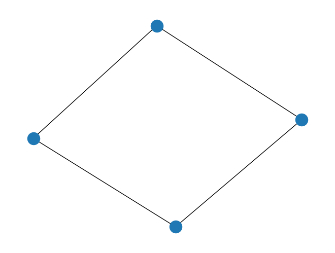
Looking at the connectivity graph, we can see that it is still possible to go from one side of the box to the other, just not directly. Intuitively, we can see that we just have to go around the obstacle.

gcs.draw()

Let’s use graph theory to find a path!

from semantic_world.spatial_types import Point3

start = Point3(-0.75, 0, 0.15)
goal = Point3(0.75, 0, 0.15)
path = gcs.path_from_to(start, goal)
print("A potential path is", [(point.x, point.y) for point in path])

A potential path is [(Expression(casadi_sx=SX(-0.75)), Expression(casadi_sx=SX(0))), (Expression(casadi_sx=SX(-0.25)), Expression(casadi_sx=SX(-0.625))), (Expression(casadi_sx=SX(0.25)), Expression(casadi_sx=SX(-0.625))), (Expression(casadi_sx=SX(0.75)), Expression(casadi_sx=SX(0)))]

This minimal example demonstrates a concept that can be applied to the entire belief state of the robot. Let’s load a more complex environment and look at the connectivity of it.

import os
from pathlib import Path
from semantic_world.adapters.urdf import URDFParser
root = next(
    parent
    for parent in [Path.cwd(), *Path.cwd().parents]
    if (parent / "pyproject.toml").exists()
)

apartment = os.path.realpath(os.path.join(root, "resources", "urdf", "kitchen.urdf"))

apartment_parser = URDFParser.from_file(apartment)
world = apartment_parser.parse()

search_space = BoundingBoxCollection([BoundingBox(min_x=-2, max_x=2,
                           min_y=-2, max_y=2,
                           min_z=0., max_z=2, origin=TransformationMatrix(reference_frame=world.root))], world.root)
gcs = GraphOfConvexSets.free_space_from_world(world, search_space=search_space)

Scalar element defined multiple times: limit

We can now see the algebraic representation of the occupied and free space. The free space is the complement of the occupied space.

from plotly.subplots import make_subplots

fig = make_subplots(rows=1, cols=2,  specs=[[{'type': 'surface'}, {'type': 'surface'}]], subplot_titles=["Occupied Space", "Free Space"])

occupied_traces = gcs.plot_occupied_space()
fig.add_traces(occupied_traces, rows=[1 for _ in occupied_traces], cols=[1 for _ in occupied_traces])
free_traces = gcs.plot_free_space()
fig.add_traces(free_traces, rows=[1 for _ in free_traces], cols=[2 for _ in free_traces])
fig.show()

Now let’s look at the connectivity of the entire world!

gcs.draw()

We can see that all spaces are somehow reachable from everywhere besides one isolated region! Amazing! This allows the accessing of locations using a sequence of local problems put together in an overarching trajectory! Finally, let’s find a way from here to there:

start = Point3(-0.75, 0, 1.15)
goal = Point3(0.75, 0, 1.15)
path = gcs.path_from_to(start, goal)
print("A potential path is", [(point.x, point.y, point.z) for point in path])

A potential path is [(Expression(casadi_sx=SX(-0.75)), Expression(casadi_sx=SX(0)), Expression(casadi_sx=SX(1.15))), (Expression(casadi_sx=SX(-0.677213)), Expression(casadi_sx=SX(0.486482)), Expression(casadi_sx=SX(1.43415))), (Expression(casadi_sx=SX(-0.677198)), Expression(casadi_sx=SX(0.486482)), Expression(casadi_sx=SX(1.43415))), (Expression(casadi_sx=SX(-0.6675)), Expression(casadi_sx=SX(-0.650005)), Expression(casadi_sx=SX(1.18405))), (Expression(casadi_sx=SX(-0.66561)), Expression(casadi_sx=SX(-0.650005)), Expression(casadi_sx=SX(1.18405))), (Expression(casadi_sx=SX(-0.60001)), Expression(casadi_sx=SX(0.674997)), Expression(casadi_sx=SX(1))), (Expression(casadi_sx=SX(0.75)), Expression(casadi_sx=SX(0)), Expression(casadi_sx=SX(1.15)))]

Known limitations and potential improvements are:

• The connectivity graph currently calculates its edges by using an approximation to adjacent surfaces. This can be improved by an exact calculation.

• The path is generated through the center points of the connection boxes. This is perhaps not optimal

• The path is chosen by taking the shortest (meaning the least amount of edges) path. This is not necessarily the best path